Computed Tomography (CT) 촬영의 원리
1. Computed Tomography란?
CT 장비는 아래 그림과 같이 내부 상태를 알고자 하는 부위를 회전축으로 하여 장비를 회전시키며 다양한 각도에서 X-Ray를 찍는다. 획득된 여러 X-Ray 정보를 합성하여 내부의 상태를 알아내는 것이 CT 촬영이다.
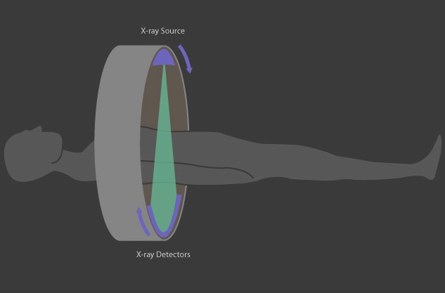
X-Ray를 회전하면서 촬영하면 왜 내부의 정보를 정확하게 알 수 있는 것일까?
X-Ray 촬영은 Figure 1과 같이 X-Ray가 투과하면서 감쇄되는 값을 측정하는 것이다. (네모 안의 값이 감쇄 값)
하나의 방향에서만 X-Ray 촬영을 하면 투과한 모든 물질의 감쇄 값 합을 알 수 있을 뿐 물질의 위치나 물질 각각의 감쇄 값을 알지 못한다.
즉 Figure 1의 (a)와 (b)는 X-Ray 촬영 결과에선 동일하게 보인다.
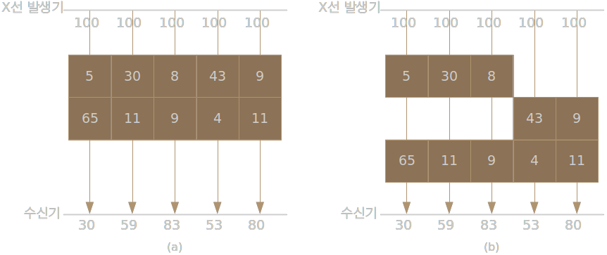
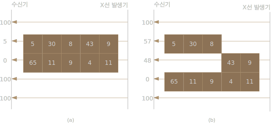
하지만 X-Ray 장비를 회전 시켜서 물체를 다른 각도로 촬영하면 Figure 1과는 다르게 (a)와 (b)의 촬영 결과는 달라지게 된다.
즉 CT는 X-Ray 촬영을 여러 각도에서 수행하여 다양한 정보를 수집하고 그 정보를 조합하여 물체 내부의 영상을 추출하는 방식이다. 정보를 조합하는 방법은 아래에서 수학적으로 설명한다.
2. 수학적 접근
2.1. Radon transform
CT의 원리를 수학적으로 풀어보기 위해서는 먼저 물체를 투과한 X-Ray 신호를 수학적으로 정의하여야 한다. 위의 그림들로 유추해 보면 X-Ray 촬영은 간단한 선적분인 것을 알 수 있다. 하지만 CT의 경우 X선 발생기의 회전도 변수로 추가되어야 하므로 선적분 함수에 회전 변수가 추가되어야 한다. 이런 함수를 Radom transform이라고 부른다.
먼저 Figure 3과 같이 축을 정의한다.
\[\begin{matrix} x=u\cos \theta -v\sin \theta \\y=u \sin\theta + v \cos\theta \end{matrix}\]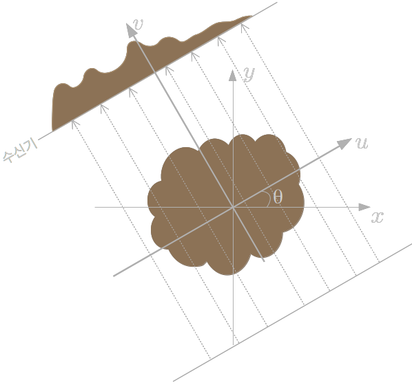
수신기에서 수집한 신호를 $p\left(u,v\right)$로 정의하면 아래와 같다.
\[p\left(u,v\right)=\int _{ -L }^{ L }{ g\left( x\left( u,v \right) , y\left( u,v \right) \right) dv }\]$p\left(u,v\right)$은 다음과 같이 각도와 $u$의 함수로 나타낼 수 있다.
\[p\left( u,\theta \right) =\int _{ -L }^{ L }{ g\left( u\cos \theta -v\sin \theta , u \sin\theta + v \cos\theta \right) dv }\]2.2. Fourier slice theorem [2]
Radon transform으로 얻어진 함수 $p\left(u, \theta\right)$를 $u$에 대해서 Fourier transform 한 결과 $P(U,\theta)$는 g(x, y)의 2D Fourier transform을 Polar Grid에서 본 것 과 같다.
먼저 random transform결과에 Fourier transform을 적용하면 다음과 같다.
\[P\left( U,\theta \right) =\int { p\left( u,\theta \right) { e }^{ -jUu }du }\]$g\left(x, y\right)$를 Fourier transform을 Polar Grid $\left(U, \theta\right)$로 출력하면 다음과 같다.
\[G\left( U\cos \theta ,U\sin \theta \right) =\iint { g\left( x,y \right) } { e }^{ -jU\cos \theta x}{ e }^{ -jU\sin \theta y}dxdy\]$x, y$를 $u, v$로 치환하면 아래와 같이 random transform이후 u축에 대한 Fourier transform으로 정리된다.
\[G\left( U\cos \theta ,U\sin \theta \right) =\iint { g\left( u\cos \theta -v\sin \theta ,u\sin \theta +v\cos \theta \right) } e^{ -jUu }dudv\] \[=\int { \left( \int { g\left( u\cos \theta -v\sin \theta ,u\sin \theta +v\cos \theta \right) dv } \right) { e }^{ -Uu }du }\] \[=\int { \left( \int { p\left( u,\theta \right) } \right) { e }^{ -Uu }du }\] \[=P\left(U, \theta \right)\]2.3. Convolution backprojection
2D Fourier transform data가 있다면 2D inverse transform을 이용하면 쉽게 데이터를 복원 할 수 있다. CT 수신 신호를 $u$축에 대해서 Fourier transform하면 $g$함수의 2D Fourier transform data를 얻을 수 있지만 Polar grid에서 얻어지게 되므로 영상으로 복원하기 위해서는 약간의 연산이 더 필요해진다.
2D Fourier transform 데이터가 직각 좌표계$\left(U,V\right)$였다면 다음과 같이 간단한 Inverse fourier transform으로 $g$를 구할 수 있을 것이다.
\[g\left( u\cos \phi ,u\sin \phi \right) =\iint { G\left( U,V \right) } { e }^{ ju\cos \phi U }{ e }^{ ju\sin \phi V }dUdV\]하지만 얻을 수 있는 데이터가 Polar grid이므로 적분 수식을 다음과 같이 변경하여야 한다.
\[g\left( u\cos \phi ,u\sin \phi \right) =\int _{ -\pi /2 }^{ \pi /2 }{ \left( \int _{ -\infty }^{ \infty }{ G\left( U\cos \theta ,U\sin \theta \right) } {\left| U \right| e }^{ ju\cos \phi U\cos \theta }{ e }^{ ju\sin U\sin \theta }dU \right) d\theta }\] \[=\int _{ -\pi /2 }^{ \pi /2 }{ \left( \int _{ -\infty }^{ \infty }{ G\left( U\cos \theta ,U\sin \theta \right) } { \left| U \right| e }^{ juU\cos \left( \phi -\theta \right) }dU \right) d\theta }\]Polar grid 적분을 위해서 Jacobian matrix에 의해서 추가된 $\left|U\right|$는 주파수 영역에서 Filtering, 영상 영역에서는 Convolution으로 해석 될 수 있다. 그래서 위와 같은 변환을 filtered backprojection 혹은 Convolution backprojection이라고 부른다.
정리하면 신체를 투과한 X-ray 자료를 각도 별로 수집하고 그 data를 Fourier transform 한다. Fourier transform된 data에 Convolution backprojection을 적용하면 신체 내부의 정보를 얻을 수 있게된다.
3. 예제 코드
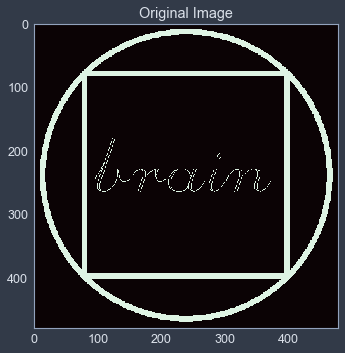
3.1. 원본 이미지
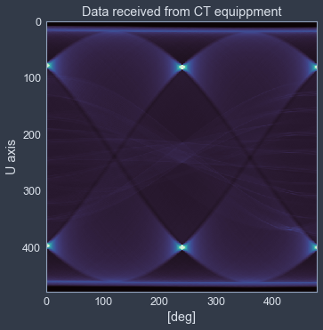
3.2. CT 장비에서 수집한 신호
from skimage.transform import radon
from numpy import linspace

n_size = 480
theta = linspace(0, 180, n_size, endpoint=False)
data_ct = radon(img, theta=theta)

jtplot.style(jtstyle)
fig, ax = subplots(nrows=1, ncols=1)
ax.imshow(data_ct, cmap=colormap)
ax.set_title("Data received from CT equippment")
ax.set_ylabel("U axis")
ax.set_xlabel("[deg]")
ax.grid(False)
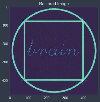
3.3. 복원한 이미지
from skimage.transform import iradon

img_restored = iradon(data_ct)

jtplot.style(jtstyle)
fig, ax = subplots(nrows=1, ncols=1)
ax.imshow(img_restored, cmap=colormap)
ax.set_title("Restored Image")
ax.grid(False)
4. 참고문헌
[1] https://www.medicalradiation.com/types-of-medical-imaging/imaging-using-x-rays/computed-tomography-ct/
[2] https://freshrimpsushi.tistory.com/1165?category=695651